Live tool: Chart comparison
BMS Chart Character Framework — Seven-Axis Radar, Tags, and Felt-Time Normalization
Subtitle: Design and validation of an analysis framework that visualizes what kind of chart a BMS chart is, rather than reducing it to a one-dimensional difficulty score.
Version: Phase 1Z final-state (YYYY-MM-DD)
This is a technical report aimed at the BMS community. It assumes basic familiarity with chart analysis and rhythm-game difficulty rating but explains every introduced term and formula in place.
Abstract
Conventional BMS difficulty labels (★, sl, st, insane-BMS, the difficulty tables) compress a chart’s demanded skill intensity into a one-dimensional scalar. But the reason a chart is hard varies enormously — some charts pressure the player with simultaneous keys, some with rapid same-lane repetition, some with tempo manipulation that disrupts perception.
This framework focuses on the character of a chart — “what kind is it hard in?” — rather than on its difficulty. The main contributions are:
- A parallel-ownership model over seven independent axes (chord / stream / scratch / soft / ln / stair / distraction): one event may contribute to multiple axes simultaneously, and the sum is not constrained to 1.
- A felt-time 1-second bucket time-axis normalization that defeats the NPS-inflation problem on BPM-trick charts.
- A dual-threshold scheme combining family-relative percentiles (p33 / p67) with absolute floors (0.03 / 0.08), preventing sparse axes from being false-flagged red on raw values.
- A three-layer card-based comparison UI (radar + tags + density bar) with a scalar-visualization invariant.
Calibration and validation were performed on a corpus of 8,555 BMS charts (SP 6,703 / DP 1,852).
1. Introduction
1.1 Problem statement
BMS chart difficulty has traditionally been expressed as a single score or single label:
- Family / scale (sl1–sl12, st0–st10, ★1–★10, ★★1–★★10, …)
- Insane / difficulty-table star ratings
- IRT (Item Response Theory) estimated chart θ
But the kind of pressure a chart applies can be:
| Pressure type | Example |
|---|---|
| Simultaneous keys (chord) | Charts with high 3+ key-press ratio |
| Sustained flow (stream) | Charts with long sustained NPS |
| Turntable (scratch) | Charts using lane 8 heavily |
| Tempo change (soft / soflan) | Charts with frequent BPM modulation |
| Long notes (LN) | Charts where holds dominate |
| Scale-progression (stair) | Charts with key-walking patterns |
| Cross-mechanism distraction | Streams interleaved with scratches |
Within a single sl10 cohort, chart A may be chord-heavy and chart B scratch-heavy. A one-dimensional scalar erases this.
1.2 Goal
Visualize the character snapshot — which kinds of pressure are present and how strongly. The framework’s output per chart consists of:
- Radar chart — 7-axis intensities shown as a hex polygon
- Tags (boolean flags) — sub-patterns the radar can’t carry (e.g. visual_gimmick, last_killing, double_tab)
- Density bar — per-second NPS over chart felt-time
1.3 Contributions
- C1 Parallel-ownership 7-axis model — one event can contribute to multiple axes; the ratios do not sum to 1
- C2 Felt-time 1-second bucketing (Z4) — kills BPM-trick NPS inflation (8,000 NPS → 449 NPS for the worst case)
- C3 Family-relative + absolute-floor dual threshold — prevents false-red on sparse axes
- C4 Scalar ↔ visualization invariant in the comparison UI — table column values match what the user can verify from the per-card visualization
2. Background
2.1 BMS chart structure
BMS is a text-based chart format. This section defines terms used later.
- Lane (line / channel) — Key position. 7-key SP uses lanes 1–7 plus a scratch (turntable) lane, typically lane 8 or “S”. DP uses 14 keys plus two scratches.
- Note — An input cue at a (lane, time) position.
- Tap — instant key press
- Long Note (LN) — a held key, with start and end events
- Tick — time unit. Independent of
#PLAYLEVEL, expressed as slot index within a#xxxNNline (measure N, channel). - Measure — musical measure. Default
4/4 = 192 ticks. #xxxNN02— per-measure length multiplier. e.g.#xxx02:0.5halves that measure. Core mechanism of measure-scale tricks.- BPM — beats per minute.
#BPM xxx(global) or#BPMxx(per-measure change). #STOP— pause measure. Usually for short stutter.#WAVkeysound — audio sample slot id each note triggers.- Chord — multiple lane notes at the same tick.
2.2 Measurement difficulty
Naïve NPS computation breaks down on BMS due to:
Class A — uniform BPM trick: Whole-chart BPM is unrealistically high (e.g. 9,999,999). Time is compressed and NPS inflates into the thousands.
Class B — segment BPM trick: One section of the chart has an unrealistic BPM. Many notes pack into that compressed segment.
Class D — measure-scale trick: #xxxNN02:1000 etc. stretches a measure to 1,000× length, packing notes into it. BPM stays normal but per-measure NPS inflates.
#STOP: Frequent short stops distort mean NPS.
This framework acknowledges these mechanisms and applies felt-time correction (§5).
2.3 Existing metrics
- NPS (Notes Per Second) — chart total notes ÷ chart length. Mean value. Inflated on Class A.
- IRT-based θ — Bayesian estimate from player clear/fail statistics. Estimates clearability, not character.
- Family / scale — curated label bundles. Two separate families: sl < st (satellite scale) and ★ < ★★ (overjoy scale). Roughly sl ≈ ★ and st ≈ ★★, with ★20 onward overlapping the start of ★★1.
2.4 Framework stance: difficulty ≠ character
This framework is intentionally decoupled from IRT clear-difficulty. Within the same family cohort, the Spearman correlation between sum-of-axes and IRT EASY-clear difficulty is ~ 0.105, very weak. Specifically:
- Axes = “what kinds of pressure does this chart have” (attribute strength)
- IRT = “is this chart clearable” (clear difficulty)
These answer different questions. We do not force axes to align with IRT.
2.5 Family × tier monotonicity (empirical IRT vs NPS)
§2.4’s decoupling claim (weak within-cohort correlation) could sound as if IRT and NPS are unrelated. They are not — the two metrics move together strongly at the family × tier mean level. What is uncorrelated is only the chart-by-chart ranking within the same tier.
This section provides the empirical basis for the framework’s calibration (family-relative percentiles) and design philosophy (axes ≠ difficulty, but both grow with family/tier).
2.5.1 Method
Of 8,555 corpus charts, we analyze 5,371 SP charts with non-low-confidence IRT statistics. Each chart’s family label (e.g. sl12) is decomposed into base (sl) and tier (12). Per family, we compute tier-by-tier means of IRT EASY-clear difficulty and NPS_mean / NPS_max.
Ideal pattern: as tier increases, both metrics increase monotonically.
2.5.2 Three family classes — different monotonicity expectations
By BMS community curation convention, each family carries a different expectation of how strongly tier monotonicity holds. We identify three classes:
| Class | Meaning | Families |
|---|---|---|
| linear-rank | Tier-mean monotonic + within-tier rank stable | SP: sl, ★ / DP: DPsl, ★ |
| body-linear-top-break | Body (lower ~3/4) monotonic, top tier admits specialist scatter | SP: st, ★★ / DP: DPst, ★★ |
| mean-tracking | Tier mean monotonic only; within-tier rank assumed noisy | SP: so, sn |
2.5.3 Empirical data
[Figure 1] SP family × tier monotonicity. Left → right: mean IRT EASY-clear · NPS_mean · NPS_max by tier. Colour encodes family, line style encodes class (linear-rank solid bold / body-linear solid / mean-tracking dotted).
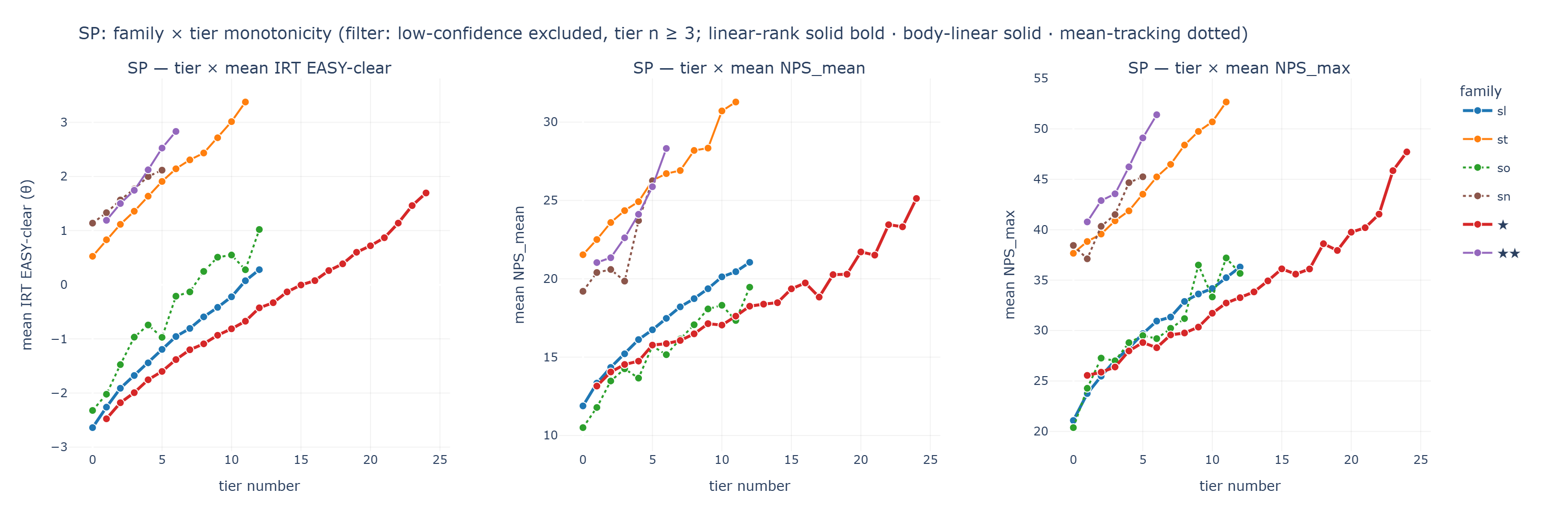
→ Interactive HTML: /Resource/Framework/figures/family_tier_monotonicity_SP.html (hover for per-tier n and values)
[Figure 2] DP family × tier monotonicity. Same layout. The DP corpus is smaller (n = 1,852), so the tier ranges are shorter, but the same monotonic pattern holds.
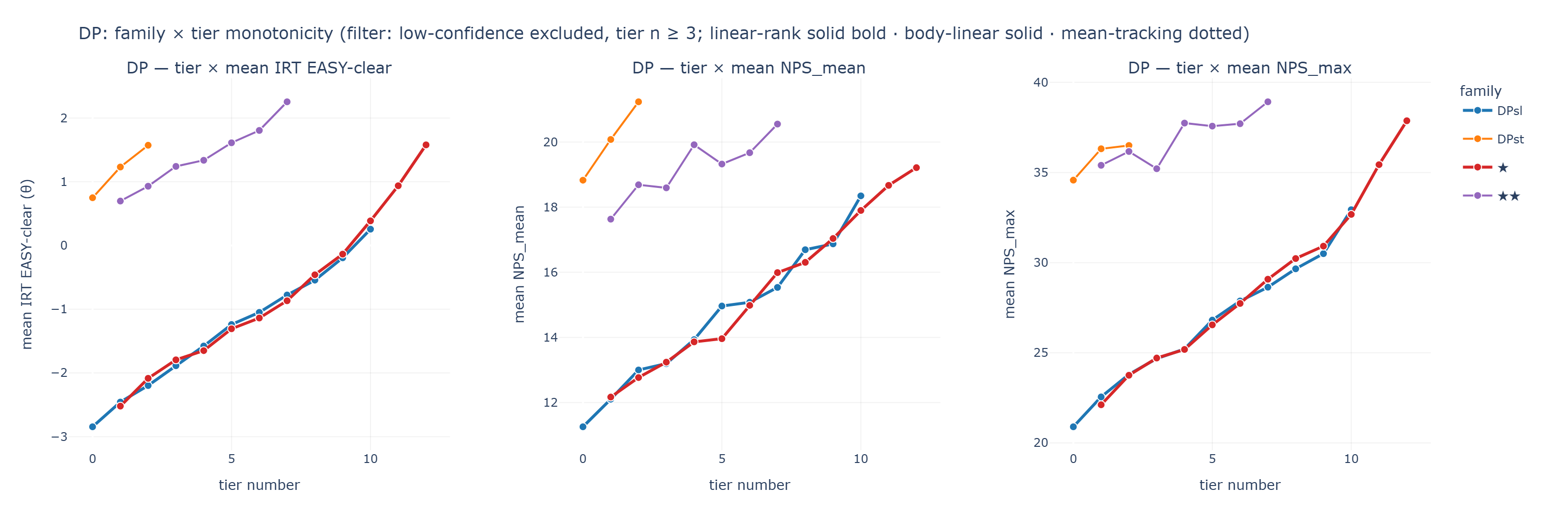
→ HTML: /Resource/Framework/figures/family_tier_monotonicity_DP.html
Regenerate: python paper/plot_family_tier.py --mode both --png
linear-rank — sl (tiers 0–12, n = 1,965)
| tier | n | IRT EASY | NPS-mean | NPS-max |
|---|---|---|---|---|
| 0 | 238 | −2.64 | 11.88 | 21.08 |
| 3 | 167 | −1.68 | 15.21 | 27.03 |
| 6 | 132 | −0.96 | 17.47 | 30.94 |
| 9 | 109 | −0.42 | 19.37 | 33.62 |
| 12 | 160 | +0.28 | 21.05 | 36.31 |
Both IRT and NPS are strict monotonic. Tier-by-tier deltas are consistent.
linear-rank — ★ (tiers 1–24, n = 952)
| tier | n | IRT EASY | NPS-mean | NPS-max |
|---|---|---|---|---|
| 1 | 47 | −2.48 | 13.15 | 25.55 |
| 6 | 47 | −1.38 | 15.86 | 28.30 |
| 12 | 57 | −0.43 | 18.25 | 33.26 |
| 18 | 28 | +0.39 | 20.26 | 38.61 |
| 24 | 7 | +1.70 | 25.13 | 47.71 |
Monotonic over all 24 steps. The longest dynamic range.
body-linear-top-break — st (tiers 0–11, n = 1,921)
| tier | n | IRT EASY | NPS-mean | NPS-max |
|---|---|---|---|---|
| 0 | 202 | +0.53 | 21.53 | 37.66 |
| 3 | 283 | +1.36 | 24.35 | 40.88 |
| 6 | 136 | +2.14 | 26.71 | 45.24 |
| 9 | 67 | +2.72 | 28.34 | 49.75 |
| 11 | 3 | +3.38 | 31.28 | 52.67 |
The body (tiers 0–9) is clean. The top (tiers 10, 11) collapses to n = 20 and 3 — insufficient for a stable monotonicity check. Curation convention reserves top tiers for specialist outliers, so evaluating a metric here uses a “body-monotonic, top-scatter accepted” criterion.
body-linear-top-break — ★★ (tiers 0–6, n = 264)
| tier | n | IRT EASY | NPS-mean | NPS-max |
|---|---|---|---|---|
| 1 | 45 | +1.19 | 21.03 | 40.78 |
| 3 | 61 | +1.75 | 22.61 | 43.56 |
| 5 | 29 | +2.53 | 25.88 | 49.10 |
| 6 | 5 | +2.83 | 28.32 | 51.40 |
Same pattern as st — body monotonic, top n drops.
mean-tracking — so (tiers 0–12, n = 128)
| tier | n | IRT EASY | NPS-mean | NPS-max |
|---|---|---|---|---|
| 0 | 16 | −2.32 | 10.50 | 20.38 |
| 2 | 15 | −1.48 | 13.48 | 27.27 |
| 4 | 10 | −0.74 | 13.66 | 28.80 |
| 5 | 6 | −0.97 | 15.71 | 29.50 |
| 8 | 16 | +0.25 | 17.06 | 31.19 |
| 11 | 5 | +0.28 | 17.34 | 37.20 |
| 12 | 3 | +1.02 | 19.46 | 35.67 |
The overall trend is upward, but IRT dips briefly at tier 4 → 5 (−0.74 → −0.97), and NPS-mean at tier 3 (14.25) exceeds tier 4 (13.66). Within-tier noise is large. The mean-tracking expectation says: “follow the overall trend; weak within-tier rank is acceptable.”
mean-tracking — sn (tiers 0–9, n = 41)
| tier | n | IRT EASY | NPS-mean | NPS-max |
|---|---|---|---|---|
| 0 | 9 | +1.14 | 19.20 | 38.44 |
| 2 | 6 | +1.57 | 20.59 | 40.33 |
| 4 | 6 | +2.00 | 23.71 | 44.67 |
| 5 | 4 | +2.12 | 26.25 | 45.25 |
| 6 | 2 | +2.21 | 10.52 | 23.50 |
| 9 | 1 | +3.39 | 25.91 | 55.00 |
Small sample (tier 6 n = 2) produces an obvious NPS outlier. IRT remains monotonic. Typical mean-tracking pattern.
2.5.4 Implications
This data underwrites two pillars of the framework’s design:
(a) IRT and NPS move together at the family-tier level. Treated as a whole corpus, the two have a strong Spearman correlation (> 0.85). “Axes ≠ difficulty” refers to within-tier cohort weak correlation, not to weak cross-tier correlation.
This distinction is important: the curated label (family/tier) itself already carries strong difficulty information. This framework is not an attempt to displace that label — it is an attempt to show what kind of character a chart has within its family/tier.
(b) Justification for family-relative calibration. The framework’s axis thresholds (p33/p67) are calibrated per-mode (SP/DP) without family stratification. Drawing percentiles from a non-family-stratified cohort assumes the family distribution is tier-monotonic. The data above confirms that assumption.
Concretely, the same raw axis value 0.5 appearing in both sl0 (NPS-mean 12) and sl12 (NPS-mean 21) is shown with the same visual intensity intentionally — “how strong is chord within this chart” is a ratio on top of a family-level NPS scale that is itself monotonically increasing.
(c) Matching expected monotonicity in evaluation. When evaluating the family-tier behavior of any axis metric, the right monotonicity must match the family’s class (linear-rank / body-linear-top-break / mean-tracking). Within-tier rank Spearman < 0.5 in a linear-rank family is a metric defect; the same result in a mean-tracking family is normal.
3. Architecture
3.1 Three-layer character snapshot
Per-chart output consists of three layers:
┌─────────────────────────────────────────┐
│  Radar (7 independent axes)             │
│  ─ chord, stream, scratch,              │
│    soft, ln, stair, distraction         │
├─────────────────────────────────────────┤
│  Tags (boolean flags, ~18)              │
│  ─ sub-patterns axes can't carry        │
│    (visual_gimmick, last_killing, ...)  │
├─────────────────────────────────────────┤
│  Density bar (per-second NPS timeline)  │
│  ─ time-axis intensity over chart       │
└─────────────────────────────────────────┘
3.2 Radar — parallel ownership
The 7 axes are independent detectors. One event can be a candidate for multiple axes (e.g. a chord-tier event on a scratch lane is +1 for both chord and scratch). Hence:
\[\sum_{a \in \text{axes}} r_a \neq 1\]where $r_a$ = candidate event count for axis $a$ / total event count.
Why? The earlier partition model (each event assigned to exactly one axis, $\sum r_a = 1$) structurally compressed any axis with low priority. For instance, when stream was the lowest-priority detector, stream-heavy charts always showed a small stream radar (Aleph-0 [INSANE] suffered this). Independent detection releases that compression.
3.3 Tags
Tags expose boolean sub-patterns that the radar can’t or shouldn’t carry. Examples:
visual_gimmick— soflan max intensity ≥ 5.0 AND off_base_note_count ≥ 4, indicating a BPM-trick chartlast_killing— late-chart NPS spikedouble_tab/triple_tab— keysound-id-matched chain (jack sub-class)jack_present— same-lane rapid pair count above floor
Tags do not surface cross-axis combinations (the radar already shows that). Tag scope is sub-metrics and composites only.
3.4 Density bar
A jet-colormap strip showing per-second NPS over felt-time. Color uses an absolute scale (cap = 60 NPS ≈ corpus p99), height is per-chart normalized (chart_max). So:
- Color = comparable across charts (absolute NPS level)
- Height = chart-internal profile (time-axis shape)
Hovering shows an instant sec N · V NPS tooltip.
3.5 Comparison table metrics — NPS, Pos/s, and compositeness
The comparison tool’s table sits below the cards (radar + density bar) and presents raw scalars side-by-side per chart. Columns:
| Column | Meaning | Unit |
|---|---|---|
| BPM | Header BPM, or felt-BPM-corrected effective BPM | beats/min |
| NPS min / mean / max | Raw note count inside an aligned 1-sec felt-time bucket (§5.5 Z4) | events / sec |
| Pos/s | Distinct timing positions per second (a chord = 1 position) | positions / sec |
| chord / stream / scratch / soft / ln / stair / distraction | 7-axis shape_v2 ratios (§4) | 0–1 |
| Peak | x_peak (peak_jab + peak_uppercut composite) | 0–1 |
NPS = Pos/s × avg_chord_size
NPS is a composite measurement — the raw count of lane presses within one second. Decomposed:
The same NPS can arise from very different mechanisms:
| Pattern | Pos/s | avg chord | NPS | Burden type |
|---|---|---|---|---|
| Chord wall (e.g. Skydive st4, 120 BPM, 7-key chords on every 16th) | 7 | 6.7 | 47 | endurance (same pattern repeating) |
| Varied chord-stream (e.g. FD [FOUR DIMENSIONS], 222 BPM, 3-4 chords with fast positional change) | 12 | 3.3 | 40 | pattern + speed (chasing positional shift) |
Looking at NPS alone, they are similar (~50 NPS) — Skydive is even slightly higher. But the underlying mechanics differ completely, and so does perceived difficulty (Skydive st4 vs FD st8/★★5).
Role of the Pos/s column: the user reads Pos/s alongside NPS to directly judge “is this chart big chords played slowly (low Pos/s + high NPS) vs fast positional shift with smaller chords (high Pos/s + moderate NPS)?”. The mechanism information NPS alone loses is decomposed and surfaced.
The radar’s chord axis exposes the same information in a different form (Skydive chord 0.99 vs FD 0.73), but if you want the arithmetic decomposition of NPS itself, Pos/s is the most direct read.
Limitation — within-chart uniformity assumption
Both Pos/s and avg chord are chart-wide averages. Mechanism differences between the first and second half of a chart (e.g. opens with a chord wall, ends with a single stream) collapse to one value each. The density bar’s time-axis visualization complements this with distributional information.
4. Per-axis metric design
Each subsection follows the structure: definition / formula / threshold / validation.
4.1 chord — simultaneous lanes (3+)
4.1.1 The radar’s raw value (shape_v2 ratio)
An event is a chord candidate if three or more lane notes coexist in a 16.67 ms (≈ 1/60 sec, one frame at 60 fps) window centered on it.
\[\text{cand}_{\text{chord}}(e) = \mathbb{1}\left[ |\{ e' : |t(e') - t(e)| < 16.67 \text{ ms} \}| \geq 3 \right]\] \[r_{\text{chord}} = \frac{\sum_e \text{cand}_{\text{chord}}(e)}{|E|}\]Why ≥3? The earlier ≥2 definition counted dual-taps as chords, pushing the corpus median to 0.67 — chord dominated the radar on nearly every chart. Raising to ≥3 lowered the median to 0.54 and restored radar balance. The user-perceived “fingers run out of room” pressure is felt from 3 lanes upward; this matches that intuition.
The 2-lane simultaneous rate is preserved as a sub-metric (chord_pair_rate) for drill-down.
Thresholds: SP (0.430, 0.638), DP (0.395, 0.563).
4.1.2 chord_burden_per_sec — shape-variety correction (v2.1)
Beyond the simple ratio, a per-second chord burden is computed as a difficulty-related sub-metric. The v2.1 (2026-05-01) form:
\[\text{chord_pace_per_sec} = \frac{\text{chord_positions}}{\text{chart_seconds}}\] \[\text{eff_avg_size} = 1 + (\text{avg_chord_size} - 1) \times (\alpha + (1 - \alpha) \times \text{variety})\] \[\text{chord_burden_per_sec} = \text{chord_pace_per_sec} \times \text{eff_avg_size}\]where:
- $\text{variety} \in [0, 1]$ — burden-weighted chord-shape Shannon entropy per size class, normalized. 0 = single-shape spam; 1 = every chord uses a distinct lane combination
- $\alpha = 0.4$ — irreducible single-shape load fraction. Even at variety = 0, the chord size still carries 40 % of its finger-count premium
Why shape-variety correction? Charts like UFS (Unidentified Flying Scotsman) are sl12 with 62 % full-7-chord 8th-note streams at 200 BPM. The simple pace × size formula (v2) gave chord 0.945 + stream 0.975 — saturating both axes at once. But a 7-key full-chord in SP has only one shape: there’s no pattern to memorize, just an endurance load. The shape-variety correction cuts the size premium for monotonic walls.
α = 0.4 meaning: variety = 0 (spam) → only 40 % of the size premium; variety = 1 (diverse) → 100 %. Codex-recommended floor.
4.1.3 chord-size distribution — big_to_mid
Additional sub-metric:
\[\text{big_to_mid} = \frac{|\{e : \text{chord_size}(e) \geq 5\}|}{|\{e : \text{chord_size}(e) \in \{3, 4\}\}|}\]Ratio of 5-7 chord events to 3-4 chord events. Used in the AEζηκ composite’s chord term (BM modulated). Intuition: detects bimodal chord-spacing patterns (small chords interleaved with large chords).
max_chord_size is also exported — base for the big_chord_burst tag (fires when the peak chord size is large).
4.2 stream — sustained density
Definition: An event is a stream candidate if the weighted NPS in its ±0.75-beat (1.5-beat total) window exceeds threshold.
Formula:
For each event $e$ at felt-time $t(e)$ with local BPM $b$, the window length in seconds is:
\[W(e) = \frac{0.75 \text{ beat}}{b / 60} = \frac{45}{b} \text{ sec}\]Weighted note count in the window:
\[N_W(e) = \sum_{e' : |t(e') - t(e)| \leq W(e)} w(e')\]where weights $w(e’)$ are:
- single (lone lane note): 1.0
- part of a chord: 0.6
- scratch lane: 0.0
Window NPS:
\[\text{nps}_W(e) = \frac{N_W(e)}{2 W(e)}\]Stream candidate:
\[\text{cand}_{\text{stream}}(e) = \mathbb{1}\left[ \text{nps}_W(e) \geq 8.0 \,\wedge\, e \notin \text{scratch lane} \right]\]Why this form? An earlier explicit chain detector (consecutive single-lane, n≥6, purity≥70%, CV≤0.20) failed on chord-mixed stream charts like Aleph-0 [INSANE] (14 / 1686 candidates). Switching to time-window weighted NPS lifted corpus nonzero coverage 47.6% → 98.1% and Aleph’s raw stream from 0.0083 → 0.7248. Adopted after two rounds of Codex cross-validation.
Thresholds:
SP: (0.736, 0.851)
DP: (0.813, 0.899)
4.3 scratch — turntable lane
4.3.1 The radar’s raw value (shape_v2 ratio)
Share of events on the scratch lane (SP lane 8; DP lanes 8 / 16). Simplest possible definition:
\[r_{\text{scratch}} = \frac{|\{e : \text{lane}(e) \in \text{SCR}\}|}{|E|}\]Thresholds: SP (0.020, 0.041), DP (0.008, 0.022).
Heavily family-dependent — sl / st charts include almost no scratches, while sn / ★★ SC (scratch character) charts are scratch-saturated. The absolute floor prevents sparse-family false-red.
4.3.2 Hidden sub-metrics — 3-feature scratch character
The simple ratio alone cannot distinguish the different burdens across charts with the same scratch share:
- case A — uniform scratch metronome spread across the chart
- case B — scratch bursts (3+ per second) in a few sections
- case C — sustained scratch chain (e.g. ≥ 8 sec continuous wheel work)
Three sub-features capture these mechanisms separately. They feed SC-tier validation and tag firing:
| Feature | Definition | Mechanism |
|---|---|---|
scratch_per_sec | scratch events / chart length (felt-sec) | Overall density (case A) |
scratch_burst_max_per_sec | Max scratch count in a 1-sec window | Peak intensity (case B) |
scratch_max_run_sec | Longest consecutive scratch chain in seconds (gap ≤ 0.5 sec) | Sustained run (case C) |
4.3.3 Long-Scratch (LS) sub-metric
A Long event on the scratch lane = wheel-hold, mechanically distinct from a quick wheel turn (the disc must be physically held). LS presence and complexity are tracked separately:
long_scratchtag — fires when LS count exceeds a floorcomplex_long_scratchtag — fires when other scratches are dense in the [ts − W, te + W] window around an LS (LS embedded in surrounding scratch, not isolated)
LS adds only ~ +0.013 Spearman to the axis composite in SC-tier validation (SP n=128) — below the noise floor, so it lives as a sub-metric / tag, not in the axis itself.
4.3.4 SP scratch-centric policy
In SP, scratch coinciding with chord (scratch_chord tag) belongs to the chord domain, and scratch interrupting stream belongs to the distraction domain (§4.7). The scratch axis itself only measures how much scratch is present.
DP has two scratches (P1/P2) and a different two-hand burden mechanic, so its distraction is formulated separately (§4.7).
4.4 soft — off-base BPM (tempo change)
4.4.1 The radar’s raw value
Share of events on a BPM segment that is not the chart’s base BPM (the BPM where most notes live):
\[r_{\text{soft}} = \frac{|\{e : \text{bpm}(e) \neq \text{bpm}_{\text{base}}\}|}{|E|}\]Intuition: a chart whose tempo-change sections carry many notes = a chart whose tempo changes actually affect play.
Thresholds: SP (0.012, 0.085), DP (0.011, 0.062). Sparse axis — the absolute floors (0.03 / 0.08) drive classification.
4.4.2 Determining base BPM — note-weighted
The definition of base BPM is subtle. Two candidates:
- Duration-weighted mode — the BPM occupying the longest wall-clock time
- Note-weighted longest-held — the BPM where the most notes actually live
The framework uses note-weighted. Reason: BPM-trick charts intentionally park implausible BPMs (e.g. 10^7) for long wall-clock spans, but those segments hold almost no notes. Duration-weighted would pick the gimmick BPM as base. Note-weighted picks the BPM where notes actually flow — sensible.
If #BASEBPM is in the header, use it directly. Otherwise compute via note-weighting.
4.4.3 Responsibility split with soflan and visual_gimmick tags
The soft axis and the tempo-related tags measure different things:
| Measurement | What it sees |
|---|---|
| soft axis | How many notes sit on off-base BPM (the play impact of tempo change) |
soflan tag | Count and magnitude of BPM changes (the chart’s structural soflan) |
visual_gimmick tag | Large BPM trick (max_intensity ≥ 5.0) + off_base_note_count ≥ 4 — display jumpscare presence |
A chart that fires all three: a genuine tempo-change challenge. Only soft = tempo change is well-integrated with notes but no large trick. Only soflan = BPM changes frequently but tempo-change parts have no notes (visual transitions only).
4.4.4 Limitation
The soft axis does not distinguish direction (acceleration vs deceleration). Player perception differs between speed-up and slow-down sections, but the metric treats them identically. Future-work candidate (see §9).
4.5 ln — Long Note
4.5.1 The radar’s raw value
The radar’s x_ln itself is a simple ratio — identical in form to the other axes’ shape_v2 candidate count / total events:
LNs on the scratch lane (= wheel-holds) are excluded because they are mechanically different — wheel-hold belongs to the scratch axis (§4.3), not multi-finger lock burden. Key-lane only policy (Phase 1Z, “each axis owns its own lane mechanics” principle).
Both LN start and end events count, so for a fixed LN count, longer holds slightly inflate the ratio (r_ln is the LN event share, not LN count).
Thresholds (SP / DP):
SP: (0.004, 0.013)
DP: (0.009, 0.020)
A sparse axis — the absolute floors (0.03 / 0.08) drive most classifications (§4.9).
4.5.2 Hidden sub-metrics — M1 / M2 / M3 / m_concurrent
The simple ratio above cannot fully describe LN play burden. For the same LN share (e.g. 40%):
- case A — long holds, sequentially placed. Hold, release, hold the next — simple LN.
- case B — short holds chained as a stream. LN by form, stream by feel.
- case C — long hold is active while another lane’s Taps arrive rapidly. Multiple fingers locked + busy free hand.
- case D — “wall of LN” — multiple LNs are simultaneously held; fingers run out of room.
These mechanism differences cannot be expressed as a single ratio. Five real-time (post felt-BPM correction) sub-features are computed alongside, feeding the advanced-LN detection in §4.5.3.
Let $h_e$ be the felt-time hold length of long event $e$. Hold floor: 1 frame (≈ 16.67 ms). Short/long boundary: 6 frames (≈ 100 ms).
M1 — short LN as stream (hold $\in$ [1 frame, 6 frames))
\[M_1 = \frac{|\{e : 1f \leq h_e < 6f\}|}{|E|}\]Stream-flowing short holds (case B). Short enough that release comes quickly.
M2 — long LN + tap activity (Tap-on-other-lane burden during long LN active)
\[M_2 = \frac{1}{T_{\text{long}}} \sum_{e \in \text{Tap}^*} n_{\text{locked}}(t_e) \times s_{\text{surround}}(t_e)\]where:
- $T_{\text{long}}$ = total hold time across long LNs ($h_e \geq 6f$)
- $\text{Tap}^*$ = key Taps occurring while any long LN is active
- $n_{\text{locked}}(t)$ = number of long LNs locked at time $t$ (strict interior: $t_s < t < t_e$)
- $s_{\text{surround}}(t)$ = number of non-LN Taps within ±1 sec of $t$
Intuition: how many fingers are committed ($n_{\text{locked}}$) × how busy the free hand is ($s_{\text{surround}}$), accumulated (case C).
M2 burst — max of M2 burden over any 1-sec window:
\[M_2^\text{burst} = \max_{\text{1-sec window}} \sum_{e \in \text{Tap}^*} n_{\text{locked}}(t_e) \times s_{\text{surround}}(t_e)\]M2 is the average burden; M2 burst is peak intensity.
M3 — M2 + short-LN-during-long (cases B and C overlapping)
\[M_3 = M_2 + \frac{1}{T_{\text{long}}} \sum_{e \in \text{ShortLN start}^*} n_{\text{locked}}(t_e) \times (s_{\text{surround}}(t_e) + 1)\]The demanding pattern where short LNs even begin during long-LN-active periods.
m_concurrent — multi-LN wall (case D)
\[m_{\text{concurrent}} = \frac{T_{\text{long}} - T_{\text{any-active}}}{T_{\text{any-active}}} = \mathbb{E}[n_{\text{active}}(t) - 1 \mid n_{\text{active}}(t) \geq 1]\]where $T_{\text{any-active}}$ is the union of times when at least one long LN is active. Intuition: while any one long LN is held, how many additional long LNs are simultaneously locked on average. Sequential-only = 0, always-2-held = 1, wall = large.
Case A leaves M2 ≈ 0, $m_{\text{concurrent}}$ ≈ 0. Case B drives $M_1$. Case C drives $M_2$. Case D drives $m_{\text{concurrent}}$. The four cases each leave their signature in different sub-features.
4.5.3 advanced_ln tag — midrank-percentile mean of 5 technical-pattern features
In addition to the 5 RT features, 5 advanced pattern features are computed separately to fire the advanced_ln tag (not surfaced on the radar):
| Feature | Definition | Intent |
|---|---|---|
adv_hand_imb | $\frac{|n_L - n_R|}{n_{\text{long}}}$ | Left/right LN imbalance |
adv_rel_pressure_1beat | Fraction of long LNs followed within ≤ 1 beat by a non-LN Tap | “release-then-jab” pressure |
adv_ln_hold_min_beats | Shortest LN hold in authored beats — inverted | Extremely short hold = harder |
adv_ln_chord_big_rate | Fraction of LN-start positions that are part of a ≥3-LN simultaneous start | Stacked LN chord (multi-finger commitment) |
adv_ln_scatter_cv | Coefficient of variation of LN inter-event gaps | Irregular scatter |
advanced_ln score = per-mode midrank percentile mean of the 5 features. Inverted features (hold_min_beats) become $1 - p$ before averaging.
Charts with no LN collapse to score = 0 (no-LN → no advanced-LN consistency). Above corpus p95, the advanced_ln tag fires.
4.5.4 Why two layers
- Radar
x_ln= “how much LN does this chart have” (user’s first question) advanced_lntag = “is the LN here technically demanding rather than just simple holds” (rarely fires, audit-worthy)
We put only the simple ratio on the radar to match the other six axes’ (chord / stream / scratch / soft / stair / distraction) shape_v2 candidate ratio form — preserving the user’s mental model. Finer LN-burden dimensions live in the tag layer.
In the current corpus (SP n = 6,703), advanced_ln fires on 0 charts — the p95 threshold is too strict, or the corpus lacks sufficiently extreme patterns. The definition is preserved so the threshold can be retuned when audit cases surface.
4.6 stair — scale-progression chains
4.6.1 Chain detection (v3 spec)
stair = chains of consecutive single notes walking adjacent lanes (±1). Captures do-re-mi-fa-style progressions like lane 1→2→3→4. Detection:
- Separate KEY-lane single notes per player (P1/P2), sort by time.
- Adjacent notes $(e_i, e_{i+1})$ belong to the same chain if:
-
lane delta $ \text{lane}(e_{i+1}) - \text{lane}(e_i) = 1$ (adjacent) - tick gap $\in [6, 12]$ — i.e. between a 16th note (6 tick) and an 8th note (12 tick)
-
- Accept chains of length $\geq 3$.
- K = 3 chord-size filter: any segment within a chain where $\geq 3$ lanes fire simultaneously is reclassified as chord, not stair. Chord-flowing-as-stair (e.g. 1+3 → 2+4 → 3+5) carries no stair character.
stair_cand collects every event participating in such a chain.
4.6.2 Burden normalization and purity factor (Phase 1V)
The shape_v2 ratio feeds the raw radar value, but two layers of normalization sit on top:
(a) p99 burden normalization:
\[\text{burden}_{\text{stair}} = \frac{\text{chain notes}}{\text{chart_seconds}}\] \[r_\text{stair}^\text{normalized} = \min(\text{burden}_{\text{stair}} / p_{99}, 1.0)\]p99 = corpus 99th percentile of burden. Extreme outliers saturate at 1.0; 99 % of charts distribute naturally below it.
(b) Purity factor (Phase 1V, 2026-05-17):
\[x_\text{stair} = r_\text{stair}^\text{normalized} \times \max(0, 1 - 0.5 \times x_\text{chord})\]When stair and chord are both strong, the stair score is deflated. Intuition: a chord-mixed stair chart (chords interleaved with stair runs) has chord burden dominating the stair burden — it is not a pure stair chart, per user audit.
Audit rationale: Empress of Raizze [フルマラソン] and Complex path [さぼてんのとげザ─] were user-perceived HIGH; Icyxis [Mystery] and 覚醒フィールド-DEATHER- were MEDIUM. Under K=3+p99 alone, all four saturated at 1.000. With the purity factor, Empress / Complex (x_chord ≈ 0.27, pure stair) read 0.865, while Icyxis / 覚醒 (x_chord ≈ 0.48, chord-mixed) read 0.744 — matching the user verdict. WF 5→8, ρ_h 0.8556→0.8653.
4.6.3 v2 L² aggregation (drill-down)
Alongside stair_burden_per_sec, a shape × fast × count 3-dimensional metric (Phase 1U) is also computed:
- shape (S): monotonic ±1 lane motion across the chain
- fast (B): chain pace vs
target_pace_per_sec = 8.0anchor - count (C): chain L² aggregation —
stair_l2 = √(Σ chain_burden²)— picks up both long single chains and many short chains
This v2 L² aggregation is a drill-down sub-metric. The radar’s raw value sits on the shape_v2 ratio.
Thresholds: SP (0.089, 0.200), DP (0.040, 0.105).
4.7 distraction — mode-split formulation
4.7.1 User-defined semantic
SP and DP have different mechanics, so they use separate formulations.
SP (one hand controls scratch + all 7 keys): distraction = quantification of scratch entering stream flow — within stream regions only, how disruptive scratches are. User intuition: “playing a stream, then scratches punch in and break flow”.
DP (two hands separated, P1 / P2 each with scratch + 7 keys): SP’s “stream interruption” framing does not transfer. DP’s strong hand independence makes user define distraction as three patterns:
- Rapid hand-role transition — LH scratch + RH keys ↔ LH keys + RH scratch, fast cycling of which hand owns the scratch role.
- Impossible scratch — same-side scratch + same-side far keys (KEY4-7) simultaneous or slightly offset. Forces the other hand onto the same side to reach those inner keys, an ergonomically unworkable placement.
- Adjacent scratch — same-side scratch + same-side near keys (KEY1-3) simultaneous or slightly offset. Playable by one hand but produces an awkward hand shape.
Responsibility split (both modes):
- Whole-chart scratch share → scratch axis (§4.3)
- Pure scratch chain (sustained run, no chord) → scratch axis’s
scratch_max_run_sec - SP scratch + chord coincidence → SP
scratch_chordtag, chord domain (§4.1) - DP chord-tier exact patterns / per-measure bilateral layout → DP-specific tags (§4.7.3)
4.7.2 SP formulation (v3 algorithm)
A 4-step pipeline on 250 ms bins:
-
Bin — every event in the chart is assigned to a 250 ms (
bin_sec = 0.25) felt-time bucket. Each bucket recordskey_count[i]andscratch_count[i]. -
Detect key-flow intervals — consecutive bins with
key_count[i] ≥ t_keyform an interval. Up togap_bins(currently 1–2) inactive bins inside are tolerated (gap-tolerant — allows brief stream pauses). -
Qualify intervals — keep only those key-flow intervals that contain at least
min_scratchesscratches. Pure key passages with no scratch contribute zero (the SP “scratches inserted into flow” framing). -
Compute v3 score:
Why the product form? A concentrated 5×5 bin × 5 occurrences carries more burden than 25 scattered 1×1 occurrences with the same total sum. Multiplication directly rewards concentration.
Why normalize by chart_seconds? Codex-recommended (2026-04-26): dividing by qualifying_sec (the total time of qualifying intervals) inflates short-flow + dense-scratch ratios. chart_seconds normalization reflects distraction load over the whole chart.
SC-tier validation (scripts/_distraction_overlap_probe_full.py):
- Shipped legacy +0.642 → v3 +0.715 (SC-tier Spearman)
-
partial scratch_per_sec: +0.354 → +0.572 (carries cross-domain signal independent of scratch density)
4.7.3 DP formulation (2-component arithmetic mean, Phase 1Z-1M)
DP x_distraction collapses §4.7.1’s three patterns (transition + impossible + adjacent) into two components, arithmetically averaged:
Component C1 — hand-role transition (alt_ratio):
Walk all scratch events in time order. For each adjacent pair $(s_i, s_{i+1})$ with time-gap $\Delta t \in [0.05, 0.30]$ s, classify:
- Different sides (P1 ↔ P2):
cross_count - Same side:
same_count
Why ratio, not rate? Rate (cross_count / chart_sec) inflates one-side-burst charts with incidental cross-side flips. $trange Attraktor [DP ANOTHER] (n=546 scratches, cross 82 / same 380): alt_ratio = 0.18 (low) but alt rate = 0.61/s (false positive). Ratio captures chart-overall hand-role balance.
Window: fixed 0.30 s (no BPM anchoring) because C1 is a motor swap concept, not “musical phrase grouping” as in C2. At 100 BPM, 1 beat is 0.6 s — too lax to call a swap. td < 0.05 (chord-tier near-simultaneous bilateral wheel) is not a transition but a bilateral chord, excluded from C1 and surfaced by the bilateral_scratch tag instead.
Component C2 — same-side scratch + key proximity (merged):
For each scratch $s$, enumerate same-side KEY1-7 events within a BPM-anchored window. Each pair contributes:
\[\frac{1}{\max(\Delta t,\ \text{chord_threshold_sec})}\]Sum, normalize by chart_seconds, clip at corpus p95 (= 7.66):
\[C_2 = \min\left(\frac{1}{\text{chart_sec}} \sum_{s \in \text{SCR}}\sum_{k \in K_s} \frac{1}{\max(\Delta t_{s,k},\ \text{chord_thresh})},\ 1.0\right)\]where $K_s$ = same-side KEY1-7 events within window of $s$.
Window: half-beat at local BPM, clamped [0.10, 0.40] s. The legacy 1-beat window was 0.46 s at 130 BPM — perceptually two separate events. Half-beat matches user’s “simultaneous or slightly offset” definition.
Why merge near (KEY1-3) / far (KEY4-7)? A compound chord (S + KEY1 + KEY5) activates both groups, causing the same scratch event to fire two components and inflate the score (~44% of $trange’s firing scratches activate BOTH near and far). The near/far distinction is preserved at the tag layer, not the axis:
DP-specific tags (chord-tier ≤ 16.67 ms exact, or per-measure pattern):
| tag | fire condition | meaning |
|---|---|---|
adjacent_scratch | same-side $S$ + KEY1-3 chord-tier count ≥ 4 | One-hand chord, awkward hand shape |
impossible_scratch | same-side $S$ + KEY4-7 chord-tier count ≥ 2 | Forces both hands onto one side |
bilateral_scratch | ≥3 scratches on each side in same measure, count ≥5 | P1/P2 wheels busy simultaneously |
4.7.4 BPM-trick handling
bpm_segments is passed in after analyze()’s felt-BPM correction (§5). So BPM-trick charts (Alcubierre Drive [INSANE], ZAKOTEMPO, etc.) get binned in felt-time correctly. DP’s local_bpm additionally falls back to effective_bpm if a stub ≥ 5× effective_bpm is hit (BPM stub trap avoidance).
4.7.5 Validation — DP 5-chart verdict set
User-labeled ground-truth set (DP, 2026-05-26):
| Chart | curator | verdict | C1 | C2 | x_distraction | corpus rank |
|---|---|---|---|---|---|---|
| P.S: Plasma Strike [GALGALIM] | DP ★ | true | 0.75 | 1.00 | 0.874 | #14 |
| キマグレ☆ [DP ANOTHER] | DP ★ | true | 0.47 | 1.00 | 0.734 | (out of samples) |
| Forceful Beat [DP HYPER] | DP ★ | true | 0.36 | 1.00 | 0.679 | #74 |
| キマグレ☆ [DP HYPER] | DP ★ | neutral ref | 0.49 | 0.21 | 0.350 | #480 |
| $trange Attraktor [DP ANOTHER] | DP ★ | false | 0.18 | 0.94 | 0.559 | #198 |
| ファンキーホット [DP INSANE] | DP ★ | false | 0.07 | 0.37 | 0.218 | #727 |
C1 (alt_ratio) is the decisive discriminator. $trange’s C2 saturates (high scratch density) but its low C1 (0.18) cleanly separates it from the true charts (0.36-0.75). 5/5 ranking matches user verdict.
Thresholds: SP (0.032, 0.084), DP (0.086, 0.290).
4.8 (Radar-out) peak, jack — drill-down only
Two metrics are computed raw but kept out of the radar:
- peak — short-window (≤ 2 sec) burden intensity (peak_jab + peak_uppercut). Cross-chart burst-severity signal.
- jack — same-lane rapid-press frequency (window = 12 ticks). Base metric for
jack_presenttag.
Excluded from the radar because peak is about burst severity rather than character, and jack is more legibly expressed as tags.
4.9 Absolute floor and the dual threshold
Each axis applies, in addition to the family-relative percentiles, an absolute floor:
- yellow ≥ max(p33, 0.03)
- red ≥ max(p67, 0.08)
Why a floor? Sparse axes (LN, soft) have very low p33/p67 (e.g. LN p67 = 0.013). Without a floor, a chart with raw value 0.015 (low absolute share) reads red. From a user’s perspective, “is this chart LN-heavy?” should not be answered “yes” when the LN share is 1.5%. The floor blocks this.
Dense axes (chord, stream, stair, distraction) have p67 well above the floor, so the floor is inert. The floor’s practical effect is on sparse axes only.
5. Felt-time normalization
This is the section that consumed the most design effort. Any attempt to correctly measure BMS chart time and density collides with the many ways chart authors play games with the time axis itself. We identify four classes of such trickery and apply different handling to each.
5.0 Order of operations
Before measuring chart time or density, the following corrections are applied in order:
Raw chart
    ↓
[A] BPM offset translation   (§5.1)
    — strip shared 10^k offset from all BPMs
    ↓
[B] Stage 1: Class B truth recovery   (§5.2)
    — pin only the gimmick segments to truth_bpm
    ↓
[C] Stage 2: Class A H1 fallback   (§5.3)
    — if Stage 1 didn't apply and triggers fire, scale all BPM down
    ↓
[D] Z4 1-sec felt-time buckets   (§5.5)
    — compute NPS on the corrected time axis
Class D (measure-scale trick) does not receive felt-BPM correction — its mechanism is different (§5.4).
5.1 [A] BPM offset translation
Mechanism
A #BPM header or #BPMxx command writes a meaningful BPM plus a large offset. For example, an actual 60-BPM section can be encoded as #BPM 10000060, which the BMS player interprets as 10 million BPM and compresses all notes into microseconds.
Detection rule
If every BPM used in the chart (base + every #BPMxx) shares the same 10^k offset, and the residual after subtraction lies in a plausible range (roughly 30 – 1500), the offset is subtracted.
Example: シャトルラン [Hexagon]
Raw BPM sequence:
  10000060, 10000064, 10000069, ..., 10000573  (linear ramp 60 → 573)

Detection: every BPM shares 10^7 offset, residuals ∈ [60, 573] all plausible
Action: subtract offset → reinterpret as 60, 64, 69, ..., 573 BPM

Result:
  effective_bpm: 101 (note-weighted mean of the linear ramp)
  chart_seconds: 138.8 sec (normal song length)
  Z4 nps_max: 7.0 (normal sn-tier flow)
Without this step, the effective BPM would be measured in the millions and every downstream metric becomes meaningless.
Example: ZAKOTEMPO
Raw: 10000199 ~ 10000277 (10^7 + [199, 277] variation)
After subtraction: 199 ~ 277 BPM, effective_bpm = 199
chart_seconds: 130.5 sec
Limits
BPM offset translation cannot fix mechanisms outside the #BPMxx line (#xxxNN02 measure scale, layered #STOP). The two charts above show residual artifacts in felt-time bucket count (e.g. シャトルラン bucket_count = 8.8M — most notes land in corrected time, but some microsecond-residual segments dominate the felt-time span). The residual does not affect NPS_max (1-sec bucket granularity), but it does distort chart-length statistics.
5.2 [B] Stage 1 — Class B truth recovery (segment trick)
Mechanism
Part of the chart is at an implausible BPM, the rest is normal. Example: the chart runs at 250 BPM but a single measure m204 is set to BPM 9,990,400, blowing past it in microseconds with notes packed in.
This form has a real BPM (truth_bpm) embedded in the chart. The duration-weighted mode BPM is in the plausible range, and most of the chart runs at it.
Detection rule (all must hold)
- Duration-weighted mode BPM ∈ [30, 1500] (plausible)
- Note-weighted effective BPM is ≥ 5× the mode BPM (divergence)
- Effective BPM itself is ≥ 1000 (implausibly high)
When all three hold, truth_bpm = duration-weighted mode BPM. Only the gimmick segments that diverge from truth are pinned to truth_bpm; normal segments are kept as-is.
Example: Alcubierre Drive [INSANE]
Raw BPM segments (roughly):
  base 174 BPM + some #BPMxx at 1.74M
  + measure_scale (xxxNN02:0.001-class) on some measures
  + ~26,000 #STOP commands (micro-stops)

Note-weighted effective BPM:
  effective_bpm ≈ 1.66M (gimmick segments dominate because notes concentrate there)

Duration-weighted mode BPM:
  174 (occupies the longest aggregate time)

Detection:
  mode=174 ∈ [30, 1500]  ✓
  effective/mode = 1.66M / 174 ≈ 9540 ≥ 5  ✓
  effective = 1.66M ≥ 1000  ✓

Action: pin every 1.66M segment to 174 (normal 174 segments stay)

Result:
  effective_bpm: 174 (recovered)
  Z4 nps_max: 33 (normal sl9 level)
  NPS_mean: 16.5 (near corpus median)
The chart header’s BPM (174) matches the recovered truth_bpm — the framework structurally recovered the chart’s actual intent (an honest 174 BPM chart) without depending on the header.
Counter-example: Aleph-0 [INSANE]
Note-weighted effective BPM: 277.8
Duration-weighted mode BPM: ~250

condition 1 (mode plausible):     250 ∈ [30, 1500]   ✓
condition 2 (5× divergence):      277.8 / 250 ≈ 1.11     ✗
condition 3 (effective ≥ 1000):   277.8 < 1000            ✗
Aleph-0 is not a BPM-trick chart — every BPM segment stays inside the plausible musical range, and the gap between effective and mode (1.11×) is a small musical variance (the denser sections sit on a slightly higher BPM than the chart-average), not a structural trick. Truth recovery requires both ≥5× divergence and effective ≥ 1000; neither holds, so the chart is analyzed at its raw BPM.
Some BMS versions of this chart reportedly contain a single-measure microsecond segment (e.g. m204 at BPM 9,990,400), but with the corpus distribution here the overall effective BPM stays under 1000, so truth recovery still does not fire. Any such single-shot burst is absorbed downstream by Z4 (§5.5) via the 1-second felt-time bucket.
5.3 [C] Stage 2 — Class A H1 fallback (uniform trick)
Mechanism
The entire chart runs at an implausible BPM. Unlike Class B, there is no embedded real BPM. Every signal is gimmick, so truth recovery cannot fire.
Detection (both triggers must fire)
- Note-weighted effective BPM >
trigger_eff_bpm(currently 500) - Declared
peak_local_max_density_per_sec>trigger_peak_per_sec(currently 200)
Action (H1 heuristic)
Uniformly scale every BPM down by the ratio declared peak NPS / target peak NPS. Target = 50 NPS (realistic peak for a hard chart).
\[\text{scale} = \frac{\text{target peak per sec}}{\text{declared peak per sec}}\] \[\text{felt_bpm} = \max(\text{declared_bpm} \times \text{scale}, \text{felt_bpm_floor})\]Floor = 30 BPM (anything lower would imply an unrealistically slow chart).
Example: シャトルラン Hexagon (counterfactual: what if [A] failed)
Hypothesis: BPM offset translation did not apply
  declared BPM: 10000060 ~ 10000573
  declared peak NPS: 800 NPS (atop 10M BPM)

  effective BPM > 500 ✓
  peak per sec > 200 ✓
  → H1 fires
  scale = 50 / 800 = 0.0625
  felt_bpm = 10M × 0.0625 ≈ 625,000 → still unrealistic

After [A] applied first, BPM is back to 60-573:
  effective BPM = 101
  peak per sec in normal range
  → H1 does not fire (conditions not met)
The order matters — [A] must clean the BPM space first so [B] and [C] operate on meaningful values.
Example: ネグラドルナ-class [MODEL 8+]
header BPM: 2222
effective BPM: ~2200 (uniform)
duration-weighted mode BPM: 2222 (out of plausible range)

Stage 1 truth recovery does not fire (mode BPM out-of-plausible)
Stage 2 H1 fires:
  scale = 50 / declared_peak ≈ 0.1
  felt_bpm = 2222 × 0.1 ≈ 222 → above floor, adopted

Result: measured as a 222 BPM chart
5.4 Class D — measure-scale trick (no felt-BPM correction)
Mechanism
#xxxNN02:k scales a measure’s length by k. BPM is normal, but k=0.001 means that measure is only 0.001 of a full measure → its notes are compressed into microseconds. Conversely k=1000 lets you stuff 1,000× more notes into a measure that still occupies its real time slot.
Why felt-BPM correction cannot help
The BPM itself is normal (e.g. 155). The felt-BPM heuristic looks at BPM, so a normal-BPM measure-scale trick never triggers it.
Tracking: scale_exposure
Note-weighted average of measure scale values is recorded as scale_exposure. Exposure ≥ 0.05 flags the chart as having significant measure-scale-trick influence.
Example: 幽雅に咲かせ、墨染の桜 [HYPER]
header BPM: 155
effective BPM: 155 (normal)
duration-weighted mode BPM: 155 (normal)
→ Neither felt-BPM correction fires

But:
  chart_seconds: 142.5 sec
  total_events: 4846
  Z4 nps_max: 449.0  ← 449 notes inside a single felt-second
  active buckets: 140
Because Z4 measures on felt-time, when a chart genuinely packs 449 notes into a real one-second window, it reports 449 NPS. Even if a measure-scale trick crammed 5,000 events into a measure, the part of that measure that occupies the felt-time second contributes that second’s NPS.
In this sense Z4 is “correctly reporting” measure-scale tricks — 449 NPS is the chart’s real player-feel intensity (it asks the player to hit 449 keys in one second). Whether that is playable is separate; the framework only measures.
5.5 [D] Z4 — 1-second felt-time buckets
Definition
event felt-second:  s_e = tick_to_sec(t(e), sec_table)
bucket index:       b_e = ⌊s_e - s_0⌋    (s_0 = min event sec)
bucket NPS:         event count in that bucket (bucket width = 1 sec)
Why this form?
The earlier measure-level binning divided each measure’s note count by its length. When a measure-scale trick or unfixed BPM trick squishes a measure into 0.015 sec, 5 notes in it produce 5/0.015 = 333 NPS. アルスノヴァに喝采を [SUPERNOVA] previously reported 8,000 NPS — a number with no musical meaning.
1-second felt-time bucketing lays a 1-sec window on the felt-time axis and counts notes inside it. Microsecond bursts inside a bucket are bounded by the second’s real width — the number equals how many keys the player presses in that real second. Honest in player-feel units.
Effect (SP corpus)
| Statistic | Before (measure) | After (1-sec bucket) |
|---|---|---|
| median NPS_max | 100.8 | 34.0 |
| p99 | 1,177.6 | 57.0 |
| max | 8,000.0 | 449.0 |
Residual cases
- max = 449 (幽雅 [HYPER]) — limit of Class D coverage (§5.4).
- Some BPM-offset charts (シャトルラン, ZAKOTEMPO) have bucket_count in the millions — the felt-time span is distorted by residual BPM-offset artifacts, but looking at active buckets only is fine (シャトルラン active=1479, ZAKOTEMPO active=1192). NPS_max is unaffected.
6. Threshold calibration
6.1 Corpus statistics
- SP: n = 6,703 (mode-active)
- DP: n = 1,852
Per-mode nonzero distributions are sorted; p33 and p67 are extracted as corpus percentiles.
6.2 Threshold derivation
- corpus regen → each chart’s axis raw values
- per-mode nonzero distribution sorted
- p33, p67 extracted
- baked into
_AXIS_INTENSITY_THRESHOLDS_SP/DP - combined with absolute floors (0.03 / 0.08) in
_classify_axis_intensityto produce the final tier:
6.3 Drift check
On any corpus regen (even with no metric change), fresh p33/p67 are compared against the baked thresholds. ∆ < 0.001 means stable; otherwise recalibrate.
7. Case studies
Each case: (chart / family / radar / key tags / time-axis shape / commentary).
7.1 Aleph-0 [INSANE] — chord-stream dominance
- Family: ★★2
- Radar: chord and stream both red. peak_uppercut = 1.00 (corpus max).
- Tags: chord_heavy, stream_dense, dense_chart
- Density: burst cluster at sec 60–65, then a sustained 30–40 NPS plateau at sec 89–102
- Commentary: Canonical chord-heavy stream chart. The parallel-ownership model lets chord and stream both fire red. Even within the ★★ family, the sustained-burst time-axis distribution visibly stands out.
7.2 Alcubierre Drive [INSANE] — BPM trick recovery
- Family: sl9
- Radar: stream red, chord yellow
- Tags: visual_gimmick, soflan, fast_chart, dense_chart
- Density: bucket_count = 1,082 (felt-time span, BPM-trick artifact)
- NPS_max: 33.0 (sl-family p75 — not an outlier)
- Commentary: Class A BPM-trick chart (BPM 1.74M warp). After felt-BPM heuristic restores BPM to 174, Z4 1-sec bucketing measures real felt-time NPS. Within the family cohort it reads as ordinary sl9. A successful case of 1-sec felt-time bucketing defeating BPM-trick micro-burst inflation.
7.3 幽雅に咲かせ、墨染の桜 [HYPER] — measure-scale outlier
- Family: ★★8
- NPS_max: 449.0 (449 notes in a single felt-second)
- Commentary: Class D measure-scale trick.
#xxxNN02:1000-class measure multipliers fit hundreds of notes into a measure that spans only ~1 second of felt-time. Not handled by the felt-BPM heuristic (BPM itself is normal; only the measure length is unusual). A limit case of the framework.
7.4 Skydive (st4) vs FREEDOM DiVE [FOUR DIMENSIONS] (st8/★★5) — density-vs-difficulty divergence
The most intuitive illustration of the framework’s “axes ≠ difficulty” principle (§2.4). Raw table values for the two charts:
| Skydive | FREEDOM DiVE [FOUR DIMENSIONS] | |
|---|---|---|
| Curator family | st4 | st8 / ★25 / ★★5 |
| BPM | 120 | 222 |
| Chart length | 67 sec | 138 sec |
| NPS mean | 44.5 | 33.0 |
| NPS max | 57 | 56 |
| Pos/s | 7.0 | 12.0 |
| avg chord size | 6.67 | 3.33 |
| x_chord | 0.99 | 0.73 |
| x_stream | 0.96 | 0.85 |
| x_peak | 0.31 | 0.64 |
| primary_character | chord-spam | chord-shape |
The trap of reading the table alone
Looking only at NPS mean: Skydive (44.5) > FD (33.0). Max is similar. If a user treats NPS as a difficulty proxy, the perception “Skydive is harder!” arises. But the curator tier says the opposite (st4 vs ★★5, ~4–5 tier gap).
Decomposing reveals the difference
Using NPS = Pos/s × avg_chord_size (§3.5):
- Skydive: 7.0 positions/sec × 6.67 chord ≈ 47 NPS. A chord wall — full 7-chord on nearly every 16th note at 120 BPM (8 pos/sec). Single pattern, endurance chart.
- FD [FOUR DIMENSIONS]: 12.0 positions/sec × 3.33 chord ≈ 40 NPS. Rapid positional shift at 222 BPM, with varied 3–4 lane chords. A pattern + speed chart.
Same ~50-NPS class, completely different mechanics.
The radar distinguishes them correctly
The framework’s radar expresses the two mechanisms distinctly:
- Skydive: chord 0.99 (saturated) + peak 0.31 (no variety) + tag
chord-spam - FD: chord 0.73 + peak 0.64 (variety) + tag
chord-shape
So the framework’s character snapshot describes the two as different characters accurately, but the raw NPS alone hides the mechanism difference. The Pos/s column (added in Phase 1Z-1L) surfaces the NPS decomposition inside the table so the user sees the compositeness directly.
Lesson
The real difficulty gap between these charts lives in dimensions the framework does not measure (pattern recognition, sight-reading, finger discipline; the 9 unmeasured dimensions in §9.1). Inferring difficulty from NPS density alone ignores which mechanism produces that density. The honest form of difficulty assessment combines the character snapshot, the curator tier label, and the user’s own rhythm-game experience.
8. Sound-aware metrics — two levels
The framework uses, or has explored, “audio information” at two distinct levels with very different cost and limits. We separate them explicitly.
| Level | Mechanism | Cost | Status in framework |
|---|---|---|---|
| L1 — keysound id matching | Compare #WAV slot ids (do two notes trigger the same sample?) | Text parsing only (free) | ✅ Adopted — jack double_tab / triple_tab tags (§8.1) |
| L2 — audio FFT pitch | Decode WAV + pyin pitch estimation | CPU / memory / pre-cache | ❌ Rejected for stair definition (§8.2) |
L1 is in production. L2 was conceptually interesting but the hypothesis broke under empirical audit. Both are documented here for BMS-community discussion.
8.1 L1 — Keysound id matching (jack, adopted)
Hypothesis
When adjacent notes in the same lane reference the same #WAV slot id — i.e. they trigger the exact same audio sample — that chain is a keysound-anchored repetition. The author intentionally engineered a “same-sound repeat”, which the player perceives as honest perceptual jack.
Implementation
For each note $e$, let token(e) be the #WAV slot id it triggers. Adjacent same-lane notes $(e_i, e_{i+1})$ form a keysound-matched pair when:
Consecutive matched pairs forming chains of length $\geq 2$ → double_tab tag; length $\geq 3$ → triple_tab tag.
Cost
No audio decoding. Only reads the #WAV slot reference from the BMS text. Zero added cost during corpus regen.
Limits
- If the author varies
#WAVids on a same-lane repeat (e.g. 02, 03, 02, 03, …) to break sound monotony, keysound-matched does not fire. Such chains are caught instead by the lane-onlyjack_presenttag. - Same
#WAVid but different actual samples (from merged BMS packages) produces false matches. Rare but possible.
8.2 L2 — Audio FFT pitch detection (stair, explored and rejected) — motivation
The stair axis (§4.6) detects chains where lane progression walks ±1. The definition looks only at chart lane pattern — it ignores whether the keysound (#WAV) actually walks a musical scale.
User’s insight: “a real perceptual stair walks not only in lane but also in audio pitch.” The same lane walk with random keysounds gives a weaker perceptual stair. Conversely, a do-re-mi-fa progression that matches the lane walk produces the listener-anchored expectation that registers as a true stair.
Hypothesis: counting only chains where lane progression and audio progression coincide will make the stair axis align better with player perception.
8.3 L2 — Implementation (Phase 1V infrastructure)
Step 1 — keysound pitch estimation
For each #WAV slot, estimate the base pitch f₀ of the audio sample. Tool: librosa.pyin (probabilistic YIN, Hz fundamental frequency estimation). Results are cached per chart.
keysound 01.wav → f₀ = 440.0 Hz  (A4)
keysound 02.wav → f₀ = 466.2 Hz  (A#4)
keysound 03.wav → f₀ = 493.9 Hz  (B4)
...
Step 2 — per-chart pitch baseline
The p95 of all keysound f₀ values in the chart serves as a baseline; each note’s pitch is expressed relative to it. Necessary because charts vary in tonal register (synth bass vs piano), so absolute Hz comparison fails.
Step 3 — sequence score
For each adjacent note pair $(e_i, e_{i+1})$ inside a stair lane chain (§4.6 definition), check whether the sign of lane delta matches the sign of pitch delta. Per-chain match ratio is computed, then weight-averaged to a chart-level audio sequence coverage.
Formula sketch:
\[\text{audio_seq_score}(c) = \frac{\sum_{(e_i, e_{i+1}) \in c} \mathbb{1}\left[ \text{sign}(\text{lane}(e_{i+1}) - \text{lane}(e_i)) = \text{sign}(f_0(e_{i+1}) - f_0(e_i)) \right]}{|c| - 1}\]where $c$ is a chain and $f_0$ is keysound pitch.
Step 4 — coverage gate
The audio score is only adopted if the fraction of keysounds that pyin could reliably pitch-detect exceeds a threshold (candidate β = 40%). Below that (typical for drum-heavy, FX-heavy, or noisy keysounds), fall back to the lane-only definition.
8.4 L2 — Empirical audit (hypothesis partially failed)
Case 1 — Flight of the Bumblebee (熊蜂の飛行), measure 4
A canonical classical scale-walk passage. Lane-wise: clean 1→2→3→4→5→6→7. Audio pitch is not sequential — either the chart author couldn’t preserve the chromatic progression via keysounds, or they intentionally separated lane walk from musical walk.
Case 2 — Terminal Strike, measures 50–57
Lane-wise a clean stair, not zigzag — a clearly perceptual stair chart. Audio pitch was found to go in the opposite direction of the lane walk in several segments.
Conclusion
“A real stair is not necessarily audio-sequential.”
The user’s case-by-case audit broke the hypothesis. Lane progression is a sufficient condition for stair character (audio direction is independent); audio-sequential alignment is not a necessary condition.
8.5 L2 — Decision and replacement
Phase 1V audio FFT was rejected. Reverted to lane-only stair detection. Two compensating measures were adopted instead:
- K=3 chord-size filter (Phase 1U) — chain segments where ≥3 lanes fire simultaneously are reclassified as chord, not stair (§4.6).
- p99 burden normalization (Phase 1U) — raw burden (chain notes / chart length) divided by p99 to normalize stair raw values to 0–1.
These two measures alone produced sufficient user-perception agreement on the stair axis (case audit: Empress / Complex vs Icyxis / 覚醒 separated correctly).
8.6 L2 — Infrastructure preserved
The audio FFT code is not removed after rejection. Possible future re-exploration:
- Other axes (LN transitions, soft) may benefit from audio signal
- Alternative pitch detectors (CREPE etc.) could re-validate the audit cases
- Audio-based features may capture other character aspects (melodic vs percussive) the lane-only model misses
What was rejected is the hypothesis that audio FFT is essential to the stair definition, not audio FFT itself.
8.7 Lesson (both L1 and L2) — conceptual soundness does not guarantee empirical adoption
“Stair = scale progression” is perceptually very plausible. But the audit revealed that BMS authors’ composing/arranging practice does not follow that perceptual model. Metric hypotheses must be empirically verified against the chart distribution.
This case argues for explicitly displaying a perceptual-vs-empirical trade matrix when framework metrics disagree with user perception. Three possibilities — (a) the metric is wrong, (b) the perception is wrong, (c) both — should not be judged asymmetrically before evidence.
9. Limitations and future work
9.1 Framework coverage
Of 22 identified difficulty dimensions, 13 are measured (≈ 60%). The 9 unmeasured:
- Memorization — playable on first read vs requires memorization
- Endurance — chart length × sustained-load accumulation
- Lane-pattern asymmetry — same NPS, different lane distribution (e.g. 1234 vs 2345) has different pressure
- Audio cue — whether the keysound tracks the chart progression
- Sight-reading — visual layout readability
- Gimmick fatigue — cumulative cognitive load from soflan / stop
- Chord pattern entropy — same chord rate, different pattern randomness
- Pattern repetition — frequency of identical pattern recurrence
- Scratch chain difficulty — scratch-run pattern (zigzag vs straight)
Candidate future work:
- M1 chord-sequence entropy
- M2 chart duration metric
- M5 anchor jack detection
- M6 pattern repetition
- Other uses of audio FFT (see §8)
9.2 Measurement limits
- Partial coverage of Class D measure-scale trick
- Small DP family sample (n = 1,852)
- No unification with IRT (deliberate decoupling)
Appendix
A. Full metric formula reference
| Consolidates formulas from §4 / §5. All ratio metrics use the chart’s playable event count $ | E | $ as denominator. |
| Axis | Candidate condition | Ratio | Notes |
|---|---|---|---|
| chord | $|{ e’ : |t(e’) - t(e)| < 16.67 \text{ms} }| \geq 3$ | $r_\text{chord} = \sum_e \text{cand}(e) / |E|$ | 16.67 ms ≈ 1/60 sec, 3+ simultaneous lanes (§4.1) |
| stream | $\text{nps}_W(e) \geq 8.0 \wedge e \notin \text{SCR}$, $\text{nps}_W = N_W / (2W)$, $W = 45/b$ sec | $r_\text{stream} = \sum_e \text{cand}(e) / |E|$ | ±0.75 beat window, weights single=1.0 / chord=0.6 / scratch=0 (§4.2) |
| scratch | $\text{lane}(e) \in \text{SCR}$ | $r_\text{scratch} = |{e : \text{lane}(e) \in \text{SCR}}| / |E|$ | Turntable lane share (§4.3) |
| soft | $\text{bpm}(e) \neq \text{bpm}_\text{base}$ | $r_\text{soft} = |{e : \text{bpm}(e) \neq \text{bpm}_\text{base}}| / |E|$ | Off-dominant-BPM segment (§4.4) |
| ln | $\text{type}(e) = \text{LN}$ | $r_\text{ln} = |{e : \text{type}(e) = \text{LN}}| / |E|$ | Both start + end counted (§4.5) |
| stair | Length ≥ 3 chain, lane Δ = ±1, tick gap ∈ [6, 12], K=3 chord filter | $r_\text{stair} = \min(\text{burden}/p_{99}, 1.0)$, $\text{burden} = \text{chain notes}/\text{chart sec}$ | p99 normalization (§4.6) |
| distraction | Scratch events inside stream interval $S$ | $r_\text{distract} = \text{scratch}(S)/|S| \times \text{intensity}$ | v3_score, intensity reflects scratch-run length (§4.7) |
Radar-out (drill-down only)
| Metric | Definition | Notes |
|---|---|---|
| peak | peak_jab + peak_uppercut (L2 burden over ≤ 2 sec window) | Burst severity (§4.8) |
| jack | Same-lane gap ≤ 12 tick pair count / sec | Base for jack_present tag (§4.8) |
Threshold classification function
\[\text{tier}(v, p_{33}, p_{67}) = \begin{cases} \text{red} & v \geq \max(p_{67}, 0.08) \\ \text{yellow} & v \geq \max(p_{33}, 0.03) \\ \text{green} & v > 0 \\ \text{null} & v = 0 \end{cases}\]Z4 (felt-time bucket NPS)
\[s_e = \text{tick_to_sec}(t(e), \text{sec_table}), \quad b_e = \lfloor s_e - s_0 \rfloor, \quad s_0 = \min_e s_e\] \[\text{NPS}(b) = \|\{e : b_e = b\}\|\]Felt-BPM correction triggers (Stage 1 — Class B truth recovery)
All three conditions must hold to fire:
- $\text{mode_bpm} \in [30, 1500]$
- $\text{effective_bpm} / \text{mode_bpm} \geq 5$
- $\text{effective_bpm} \geq 1000$
On fire, only the gimmick segments are pinned to $\text{truth_bpm} = \text{mode_bpm}$.
Stage 2 — Class A H1 fallback
Both triggers must fire:
- $\text{effective_bpm} > 500$
- $\text{declared peak NPS} > 200$
On fire, every BPM is uniformly scaled by $\text{scale} = 50 / \text{declared peak NPS}$. $\text{felt_bpm} = \max(\text{declared_bpm} \times \text{scale}, 30)$.
B. Threshold table
                SP                       DP
chord:          (0.430, 0.638)           (0.395, 0.563)
stream:         (0.736, 0.851)           (0.813, 0.899)
scratch:        (0.020, 0.041)           (0.008, 0.022)
soft:           (0.012, 0.085)           (0.011, 0.062)
ln:             (0.004, 0.013)           (0.009, 0.020)
stair:          (0.089, 0.200)           (0.040, 0.105)
distraction:    (0.032, 0.084)           (0.086, 0.290)
peak:           (0.441, 0.608)           (0.525, 0.672)
jack:           (0.223, 0.369)           (0.265, 0.436)
absolute floors: yellow ≥ 0.03, red ≥ 0.08
C. Tag definitions (18)
Each tag’s fire condition and SP corpus (n = 6,703) fire counts. The two zero-fire tags (advanced_ln, peak_outlier) are defined in the code but never trigger on the current corpus — reserved slots for rare patterns that the user considers meaningful when they do appear.
| Tag | Category | Fire condition | SP fire | % |
|---|---|---|---|---|
burst_focused | peak | Peak burden concentrated in a small region (peak_concentration high) | 2,835 | 42.3% |
dense_chart | density | Whole-chart average NPS exceeds threshold | 2,119 | 31.6% |
big_chord_burst | chord | Peak chord size is large (many simultaneous lanes at the maximum moment) | 1,697 | 25.3% |
sustained | peak | Peak burden spread across the chart (peak_concentration low) | 1,335 | 19.9% |
jack_present | jack | Same-lane rapid pair count exceeds floor (keysound-agnostic) | 1,226 | 18.3% |
scratch_burst | scratch | Scratch flurry within a 1-sec window exceeds threshold | 845 | 12.6% |
last_killing | structural | Late-chart NPS spike (escalating finale or back-spike + calm coda) | 543 | 8.1% |
scratch_chord | cross-mech | (SP) Scratch coincides with chord-tier notes (cross-domain pressure) | 425 | 6.3% |
impossible_scratch | cross-mech | (DP) Same-side $S$ + KEY4-7 chord-tier exact (both hands forced to one side) | 130 | 7.0% DP |
adjacent_scratch | cross-mech | (DP) Same-side $S$ + KEY1-3 chord-tier exact (awkward one-hand chord) | 103 | 5.6% DP |
bilateral_scratch | cross-mech | (DP) ≥3 scratches per side in same measure, count ≥ 5 | 39 | 2.1% DP |
long_scratch | scratch | Sustained Long-Scratch (wheel-hold) presence above floor | 385 | 5.7% |
flow_break | jack | Jacks interrupt running streams at a high rate | 348 | 5.2% |
extreme_burst | density | Off-base BPM burst severity very high (BPM-scaled) | 160 | 2.4% |
double_tab | jack (keysound) | Same #WAV id 2-chain repetition present (§8.1) | 92 | 1.4% |
jack_chart | jack | Pure-jack rate per second exceeds threshold (isolated jack, outside streams) | 83 | 1.2% |
complex_long_scratch | scratch | Long Scratch embedded in other scratch context (not isolated) | 61 | 0.9% |
triple_tab | jack (keysound) | Same #WAV id 3+ chain repetition present (§8.1) | 57 | 0.9% |
visual_gimmick | gimmick | High soflan max-intensity ≥ 5.0 AND off_base_note_count ≥ 4 | 54 | 0.8% |
advanced_ln | ln | LN technical composite (short-hold transition, stacked LN chord, irregular scatter) | 0 | 0.0% |
peak_outlier | peak | Peak axis red AND sustained — high peak that doesn’t cluster | 0 | 0.0% |
D. Corpus statistics
Total charts: 8,555 (SP 6,703 / DP 1,852)
Family distribution (family-labeled charts only — un-labeled charts are still analyzed by the framework but excluded from this distribution)
SP (n = 5,738 with family / 965 no family / total 6,703):
| family | n | % of SP | class (§2.5.2) |
|---|---|---|---|
sl | 2,131 | 31.8% | linear-rank |
st | 2,033 | 30.3% | body-linear-top-break |
★ | 952 | 14.2% | linear-rank |
★★ | 347 | 5.2% | body-linear-top-break |
so | 201 | 3.0% | mean-tracking |
sn | 74 | 1.1% | mean-tracking |
DP (n = 1,735 with family / 117 no family / total 1,852):
| family | n | % of DP | class |
|---|---|---|---|
DPsl | 634 | 34.2% | linear-rank |
★ | 623 | 33.6% | linear-rank |
★★ | 343 | 18.5% | body-linear-top-break |
DPst | 135 | 7.3% | body-linear-top-break |
Charts without a family label (no-family) are charts excluded from curated classification (personal mods, unreleased, unassigned). They remain in the framework analysis but are excluded from family-relative comparisons.
IRT data: From the PL3 SP IRT result (6,103 charts), only rows with Low-sample low-confidence flag = False are used — after joining with the chart summary, 5,371 charts back the §2.5 analysis.
Mode separation: All metric calibration and thresholds are computed per mode (SP / DP). Cross-mode comparison is not intended (SP 8-key and DP 16-key have different lane mechanics).